Streaming Twitter data with Microsoft Flow and Power BI
It is already a long time ago that I wrote a blog about streaming data with the ELK stack. Today you see a lot of the so called “no code” solutions. You need only some configurations and that’s it! In this blog I use Microsoft Flow and Microsoft Power BI with the focus on streaming data.
What is Microsoft Flow?
Microsoft FLow creates automated workflows between your favorite apps and services to get notifications, synchronize flies, collect data and more. It looks like the old Yahoo Pipes which was very powerfull. The purpose of Yahoo Pipes was to create new pages by aggregating RSS feeds from different sources. Microsoft Flow has also very much in common with the very popular If This Than That (IFTT) platform. More info about Microsoft Flow here
What is Microsoft Power BI?
Power BI is a suite of business analytics tools that deliver insights throughout your organization. Connect to hundreds of data sources, simplify data prep, and drive ad hoc analysis. Produce beautiful reports, then publish them for your organization to consume on the web and across mobile devices. Everyone can create personalized dashboards with a unique, 360-degree view of their business. More info about Microsoft Power BI here
Suppose we want to create a twitter stream about a live soccer match, we can make a twitter flow in Microsoft Flow (and do a sentiment analyse on the tweet text) and finally create an action to a Power BI API stream endpoint.
Step one, we create a Power BI API endpoint:
Go to https://powerbi.microsoft.com/ and login. If you do not have an account sign up. When logged on find My Workspace → Datasets → Create (the + sign in the upper right corner)
We use the API button to create an API endpoint. Give the stream a name and create the following fields:
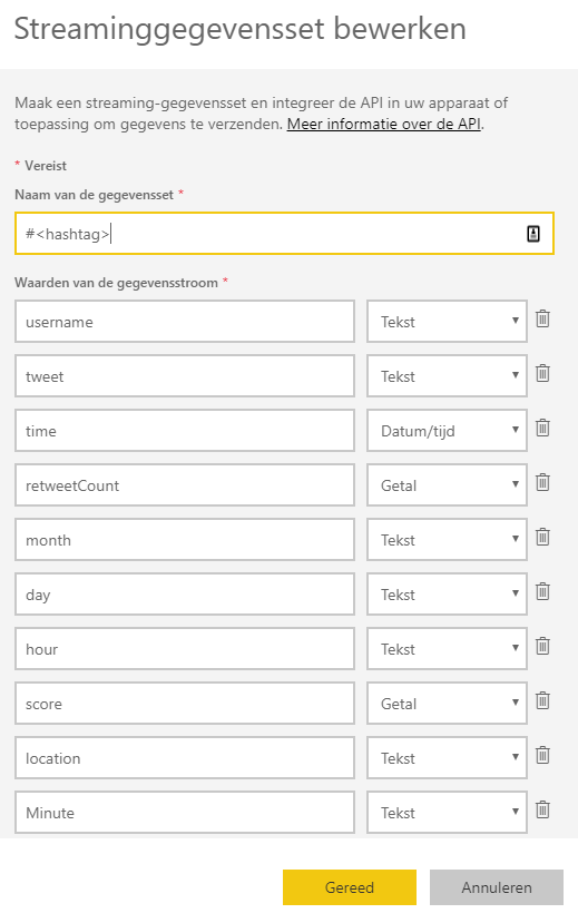
We need some extra time dimension fields month, day, hour and minute to use drill/down features later on in Power BI. The outcome of the sentiment analyse on the tweet text will be placed in the field ‘score’. From 0 to 1 is from more negative to more positive. Power BI show the following field formats.
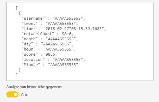
Power BI makes a JSON like format (a REST Webservice on the background). Switch ‘historical data’ to ‘on’, if you will save the data for analysis later in time. You only can access those (historical) dataset with Power BI Desktop if this switch is ‘on’.
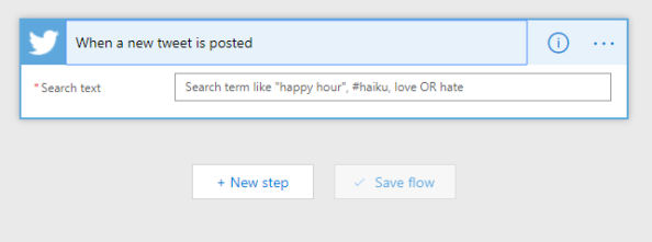
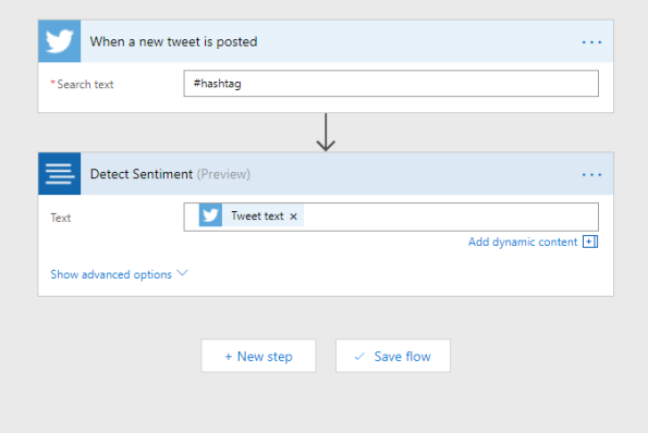
Now we go to Microsoft Flow https://flow.microsoft.com. Login (otherwise sign up for a new account) and ‘create a new flow from blank’. Find the trigger ‘When a new tweet is posted’. Enter a <hashtag>, you can also use boolean operators like ‘AND’ or ‘OR’.
In the next step we add a new action. Use the search word ‘sentiment’ and the connector ‘Text Analytics – Detect Sentiment’. Choose the ‘Tweet text’ field to fill the Text field.
Now enter the last step and add the last action to connect to Power BI. Search for ‘power bi’ in the search box and choose the Power BI connector. Fill in the workspace ‘My Workspace’ and fill in the name of the streaming dataset you give in Power BI earlier. The table field is filled with ‘RealTimeData’.
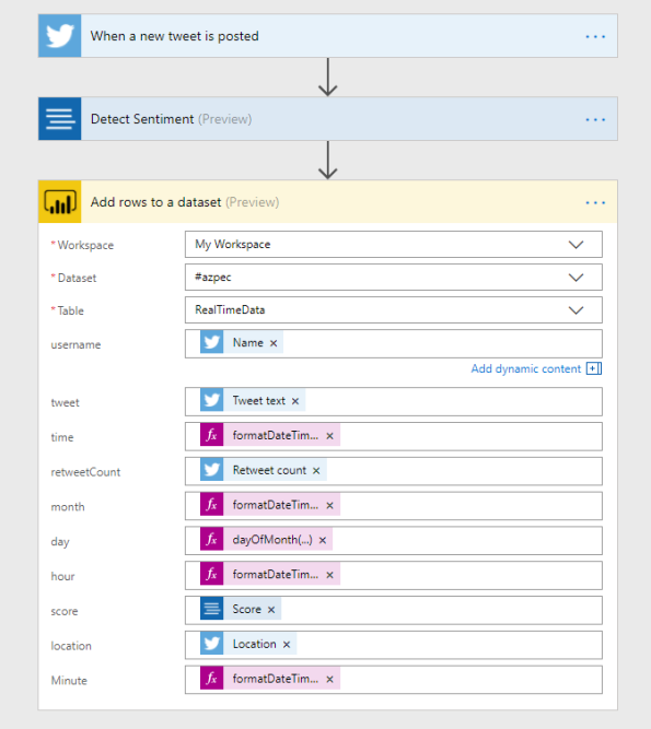
If everything is complete you see the above picture. The twitter fields and the score field of the sentiment analysis is clear. For the time fields we use expressions (I live in the timezone UTC+1).
- time = formatDateTime(addHours(utcNow(),1),’MM/dd/yyyy HH:mm:ss’)
- month = formatDateTime(addHours(utcNow(),1),’MM’)
- day = dayOfMonth(addHours(utcNow(),1))
- hour = formatDateTime(addHours(utcNow(),1),’HH’)
- Minute = formatDateTime(addHours(utcNow(),1),’mm’)
I started my flow on the 31 January 2018 around 17:00 (the start of the match was 18:30) and I used the match AZ against PEC Zwolle (hashtag #azpec) in the quarter final of the KNVB beker. Below some nice charts that I have made in Power BI.

On this charts you see the number of tweets per minute. I also use the Wordcloud chart, that you can import from the marketplace. When you press the minute bar on 18:53, you can see that Wordcloud collect all the words of the tweets that are send on minute 18:53 and we see clearly that Wout Weghorst makes the first goal!

On this chart you can see that the average sentiment around Alkmaar the home place of AZ is more positive, than the rest of the country.
Of course I can show a lot more charts to show you the power of Power BI, but I stop here … 🙂
There are some things that can be better and maybe the Microsoft Power BI team can make this happen in one of the monthly Power BI updates.
- The number of charts are limited when you use the real-time dash board of Power BI. In this blog I collect the data first to use the power of all the available charts.
- You cannot add or enrich more data to a Power BI stream. For example I want to add a time dimension (as a new relation/table) to the streaming data set.
Next time more …
Top 5 Big Data Platform predictions for 2017
The Rise of Data Science Notebooks
Apache Zeppelin is a web-based notebook that enables interactive data analytics. You can make beautiful data-driven, interactive and collaborative documents with SQL, Scala or Python and more. However Apache Zeppelin is still an incubator project, I expect a serious boost of notebooks like Apache Zeppelin on top of data processing (like Apache Spark) and data storage (like HDFS, NoSQL and also RDBMS) solutions. Read more on my previous post.
Splice Machine replace traditional RDBMSs
Splice Machine delivers an open-source database solution that incorporates the proven scalability of Hadoop, the standard ANSI SQL and ACID transactions of an RDBMS, and the in-memory performance of Apache Spark.

Machine Learning as a Service (MLaaS)
Machine Learning is the subfield of computer science that “gives computers the ability to learn without being explicitly programmed”. Within the field of data analytics, Machine Learning is a method used to devise complex models and algorithms that lend themselves to prediction; this is known as predictive analytics. The rise of Machine Learning as a Service (MLaaS) model is good news for the market, because it reduce the complexity and time required to implement Machine Learning and opens the doors to increase the adoption level. One of the companies that provide MLaaS is Microsoft with Azure ML.
Apache Spark on Kubernetes with Red Hat OpenShift
OpenShift is Red Hat‘s Platform-as-a-Service (PaaS) that allows developers to quickly develop, host, and scale applications in a cloud environment. OpenShift is a perfect platform for building data-driven applications with microservices. Apache Spark can be made natively aware of Kubernetes with OpenShift by implementing a Spark scheduler backend that can run Spark application Drivers and bare Executors in Kubernetes pods. See more on the OpenShift Commons Big Data SIG #2 blog.
MapR-FS instead of HDFS
If you’re familiar with the HDFS architecture, you’ll know about the NameNode concept, which is a separate server process that handles the locations of files within your clusters. MapR-FS doesn’t have such a concept, because all that information is embedded within all the data nodes, so it’s distributed across the cluster. The second architectural difference is the fact that MapR is written in native code and talks to directly to disk. HDFS (written in Java) runs in the JVM and then talk to a Linux file system before it talks to disks, so you have a few layers there that will impact performance and scalability. Read more differences in the MapR-FS vs. HDFS blog.
Apache Zeppelin “the notebook” on top of all the (Big) Data
Apache Zeppelin is a web-based notebook that enables interactive data analytics. You can make beautiful data-driven, interactive and collaborative documents with SQL, Scala or Python and more. However Apache Zeppelin is still an incubator project, I expect a serious boost of notebooks like Apache Zeppelin on top of data processing (like Apache Spark) and data storage (like HDFS, NoSQL and also RDBMS) solutions.
But is Apache Zeppelin covered in the current Hadoop distributions Cloudera, Hortonworks and MapR?
Cloudera is not covering Apache Zeppelin out of the box, but there is blog post how to install Apache Zeppelin on CDH. Hortonworks is covering Apache Zeppelin out of the box, see the picture of the HDP projects (well done Hortonworks). MapR is not covering Apache Zeppelin out of the box, but there is a blog post how to build Apache Zeppelin on MapR.

Is Apache Zeppelin covered by the greatest cloud providers Amazon AWS, Microsoft Azure and Google Cloud Platform?
We see that Amazon Web Services (AWS) has a Platform as a Service solution (PaaS) called Elastic Map Reduce (EMR). We see that since this summer Apache Zeppelin is supported on the EMR release page.
![]()
If we look at Microsoft Azure, there is a blog post how to start with Apache Zeppelin on the HD Insights Spark Cluster (this is a also a PaaS solution).
If we look at Google Cloud Platform we see a blog post to install Apache Zeppelin on top of Google BigQuery.
And now a short demo, lets do some data discovery with Apache Zeppelin on an open data set. For this case I use the Fire Report from the City of Amsterdam from 2010 – 2015.
If you want a short intro look first at this short video of Apache Zeppelin (overview).
I use of course docker to start a Zeppelin container. I found an image in the docker hub from Dylan Meissner (thx). Run the docker container to enter the command below:
$ docker run -d -p 8080:8080 dylanmei/zeppelin
Look in the browser at dockerhost:8080 and create a new notebook:
Step 1: Load and unzip the dataset (I use the “shell” interpreter)
%sh
wget https://files.datapress.com/amsterdam/dataset/brandmeldingen-2010-2015/2016-02-25T14:51:13/brwaa_2010-2015.zip -O /tmp/brwaa_2010-2015.zip
%sh
unzip /tmp/brwaa_2010-2015.zip -d /tmp
Step 2: Clean the data, in this case remove the header
%sh
sed -i '1d' /tmp/brwaa_2010-2015.csv
Step 3: Put data into HDFS
%sh
hadoop fs -put /tmp/brwaa_2010-2015.csv /tmp
Step 4: Load the data (most import fields) via a class and use the map function (default Scala)
val dataset=sc.textFile("/tmp/brwaa_2010-2015.csv")
case class Melding (id:  Integer, melding_type: String, jaar: String, maand_nr: String, prioriteit: String, uur: String, dagdeel: String, buurt: String, wijk: String, gemeente: String)
val melding = dataset.map(k=>k.split(";")).map(
k => Melding(k(0).toInt,k(2),k(7),k(8),k(14),k(15),k(16),k(19),k(20),k(22))
)
melding.toDF().registerTempTable("melding_table")
Step 5: Use Spark SQL to run the first query
%sql
select count(*)
from melding_table
Below you can see some more queries and charts:

Next step is how to predict fire with help of Spark ML.
Stream and analyse Tweets with the ELK / Docker stack in 3 simple steps
There are a lot of possibilities with Big Data tools on the today’s market. For example if we want to stream and analyse some tweets there are several ways to do this. For example:
- With the Hadoop ecosystem Flume, Spark, Hive etc. and present it for example with Oracle Big Data Discovery.
- With the Microsoft Stack from Azure (Hadoop) and with Power BI to Excel.
- Or with this blog with the ELK stack (see Elastic) with the help of the Docker ecosystem
- and of course al lot more solutions …
What is the ELK stack? ELK stands for Elasticsearch (Search & Analyze Data in Real Time), Logstash (Process Any Data, From Any Source) and Kibana (Explore & Visualize Your Data). More in info at Elastic.
Most of you know Docker already. Docker allows you to package an application with all of its dependencies into a standarized unit for software development. And … Docker will be more and more import with all kind of Open Source Big Data solutions.
Let’s go for it!
Here are the 3 simple steps:
- Step 1: Install and test Elasticsearch
- Step 2: Install and test Logstash
- Step 3: Install and test Kibana
For now you need only a dockerhost. I use Docker Toolbox.
If you don’t have a virtual machine, create one. For example:
$ docker-machine create --driver virtualbox --virtualbox-disk-size "40000" dev
Logon to the dockerhost (in my case Docker Toolbox)
$ docker-machine ssh dev
Step 1: Install and test Elasticsearch
Install:
docker run --name elasticsearch -p 9200:9200 -d elasticsearch --network.host _non_loopback_
The –network.host _non_loopback_ option must be added from elasticsearch 2.0 to handle localhost
Test:
curl http://localhost:9200
You must see something like:
{
  "status" : 200,
  "name" : "Dragonfly",
  "cluster_name" : "elasticsearch",
  "version" : {
    "number" : "1.7.0",
    "build_hash" : "929b9739cae115e73c346cb5f9a6f24ba735a743",
    "build_timestamp" : "2015-07-16T14:31:07Z",
    "build_snapshot" : false,
    "lucene_version" : "4.10.4"
  },
  "tagline" : "You Know, for Search"
}
Step 2: Install and test Logstash
Make the following “config.conf” file for streaming tweets to elasticsearch. Fill in your twitter credentials and the docker host ip. For this example we search all the tweets with the keyword “elasticsearch”. For now we do not use a filter.
input {
  twitter {
      consumer_key => ""
      consumer_secret => ""
      oauth_token => ""
      oauth_token_secret => ""
      keywords => [ "elasticsearch" ]
      full_tweet => true
  }
}
filter {
}
output {
  stdout { codec => dots }
  elasticsearch {
    protocol => "http"
    host => "<Docker Host IP>"
    index => "twitter"
    document_type => "tweet"
  }
}
Install:
docker run --name logstash -it --rm -v "$PWD":/config logstash logstash
 -f /config/config.conf
Test (if everything went well) you see:
Logstash startup completed
...........
Step 3: Install and test Kibana
Install and link with the elasticsearch container:
docker run --name kibana --link elasticsearch:elasticsearch -p 5601:5601 -d kibana
Test:
curl http://localhost:5601
You must see something like a html page. Go to a browser and see the Kibana 4 user interface.
Start to go to settings tab and enter the new index name “twitter”
Go to the discover tab and you see something like this (after 60 minutes):

I also make a pie chart (Tweets per Location) like this:

And there are a lot of more possibilities with the ELK stack. Enjoy!
More info:
Install single node Hadoop on CentOS 7 in 5 simple steps
First install CentOS 7 (minimal) (CentOS-7.0-1406-x86_64-DVD.iso)
I have download the CentOS 7 ISO here
### Vagrant Box
You can use my vagrant box voor a default CentOS 7, if you are using virtual box
$ vagrant init malderhout/centos7
$ vagrant up
$ vagrant ssh
### Be aware that you add the hostname “centos7” in the /etc/hosts
127.0.0.1 centos7 localhost localhost.localdomain localhost4 localhost4.localdomain4
### Add port forwarding to the Vagrantfile located on the host machine. for example:
config.vm.network “forwarded_port”, guest: 50070, host: 50070
### If not root, start with root
$ sudo su
### Install wget, we use this later to obtain the Hadoop tarball
$ yum install wget
### Disable the firewall (not needed if you use the vagrant box)
$ systemctl stop firewalld

We install Hadoop in 5 simple steps:
1) Install Java
2) Install Hadoop
3) Configurate Hadoop
4) Start Hadoop
5) Test Hadoop
1) Install Java
### install OpenJDK Runtime Environment (Java SE 7)
$ yum install java-1.7.0-openjdk
2) Install Hadoop
### create hadoop user
$ useradd hadoop
### login to hadoop
$ su - hadoop
### generating SSH Key
$ ssh-keygen -t dsa -P '' -f ~/.ssh/id_dsa
### authorize the key
$ cat ~/.ssh/id_dsa.pub >> ~/.ssh/authorized_keys
### set chmod
$ chmod 0600 ~/.ssh/authorized_keys
### verify key works / check no password is needed
$ ssh localhost
$ exit
### download and install hadoop tarball from apache in the hadoop $HOME directory
$ wget http://apache.claz.org/hadoop/common/hadoop-2.5.0/hadoop-2.5.0.tar.gz
$ tar xzf hadoop-2.5.0.tar.gz
3) Configurate Hadoop
### Setup Environment Variables. Add the following lines to the .bashrc
export JAVA_HOME=/usr/lib/jvm/jre
export HADOOP_HOME=/home/hadoop/hadoop-2.5.0
export HADOOP_INSTALL=$HADOOP_HOME
export HADOOP_MAPRED_HOME=$HADOOP_HOME
export HADOOP_COMMON_HOME=$HADOOP_HOME
export HADOOP_HDFS_HOME=$HADOOP_HOME
export HADOOP_YARN_HOME=$HADOOP_HOME
export HADOOP_COMMON_LIB_NATIVE_DIR=$HADOOP_HOME/lib/native
export PATH=$PATH:$HADOOP_HOME/sbin:$HADOOP_HOME/bin
export JAVA_LIBRARY_PATH=$HADOOP_HOME/lib/native:$JAVA_LIBRARY_PATH
### initiate variables
$ source $HOME/.bashrc
### Put the property info below between the “configuration” tags for each file tags for each file
### Edit $HADOOP_HOME/etc/hadoop/core-site.xml
<property>
  <name>fs.default.name</name>
    <value>hdfs://localhost:9000</value>
</property>
### Edit $HADOOP_HOME/etc/hadoop/hdfs-site.xml
<property>
 <name>dfs.replication</name>
 <value>1</value>
</property>

<property>
  <name>dfs.name.dir</name>
    <value>file:///home/hadoop/hadoopdata/hdfs/namenode</value>
</property>

<property>
  <name>dfs.data.dir</name>
    <value>file:///home/hadoop/hadoopdata/hdfs/datanode</value>
</property>
### copy template
$ cp $HADOOP_HOME/etc/hadoop/mapred-site.xml.template $HADOOP_HOME/etc/hadoop/mapred-site.xml
### Edit $HADOOP_HOME/etc/hadoop/mapred-site.xml
<property>
  <name>mapreduce.framework.name</name>
   <value>yarn</value>
</property>
### Edit $HADOOP_HOME/etc/hadoop/yarn-site.xml
<property>
  <name>yarn.nodemanager.aux-services</name>
    <value>mapreduce_shuffle</value>
</property>
### set JAVA_HOME
### Edit $HADOOP_HOME/etc/hadoop/hadoop-env.sh and add the following line
export JAVA_HOME=/usr/lib/jvm/jre
4) Start Hadoop
# format namenode to keep the metadata related to datanodes
$ hdfs namenode -format
# run start-dfs.sh script
$ start-dfs.sh
# check that HDFS is running
# check there are 3 java processes:
# namenode
# secondarynamenode
# datanode
$ start-yarn.sh
# check there are 2 more java processes:
# resourcemananger
# nodemanager
5) Test Hadoop
### access hadoop via the browser on port 50070

### put a file
$ hdfs dfs -mkdir /user
$ hdfs dfs -mkdir /user/hadoop
$ hdfs dfs -put /var/log/boot.log
### check in your browser if the file is available

Works!!! See also https://github.com/malderhout/hadoop-centos7-ansible
Stream Tweets in MongoDB with Node.JS
Suppose we want store al our “mongodb” tweets in a MongoDB database.
We need 2 additional node packages:
1) ntwitter (Asynchronous Twitter REST/stream/search client API for Node.js)
2) mongodb (A Node.js driver for MongoDB). Of course there are more MongoDB drivers.
Create a Node.js project “twitterstream” and add the 2 packages with the following commands:
$ npm install ntwitter
$ npm install mongodb
We need an existing twitter account and make a credential file for example credentials.js.
var credentials = {
    consumer_key: '3h7ryXnH209mHNWvTgon5A',
    consumer_secret: 'tD5OdqXw1qbDMrFbrtPIRRl4fEyUsKFXT2kZLQaMpVA',
    access_token_key: '474665342-wuRquALXNQZPYABUiOnXCmVSxyU2LIinV6VwpWMW',
    access_token_secret: 'k01HuXdl8umwt5rZcDDk0OgQJbhkiFlPv2dCAmHXQ'
};

module.exports = credentials;
And now we create the main file twitter.js with the following code:
var twitter = require('ntwitter');
var credentials = require('./credentials.js');

var t = new twitter({
    consumer_key: credentials.consumer_key,
    consumer_secret: credentials.consumer_secret,
    access_token_key: credentials.access_token_key,
    access_token_secret: credentials.access_token_secret
});

var mongo = require('mongodb');

var Server = mongo.Server,
    Db = mongo.Db,
    assert = require('assert')
    BSON = mongo.BSONPure;

var server = new Server('localhost', 27017, {auto_reconnect: true});
db = new Db('twitterstream', server);
// open db
db.open(function(err, db) {
  assert.equal(null, err);

  t.stream(
    'statuses/filter',
    { track: ['mongodb'] },
    function(stream) {
        stream.on('data', function(tweet) {
            db.collection('streamadams', function(err, collection) {
               collection.insert({'tweet': tweet.text, {safe:true}
                                 , function(err, result) {});
            });
        });
    }
  );
});
Simply start the twitter.js with:
$ node twitter.js
Succes with Node.JS and MongoDB!
How to Fetch RSS feeds into MongoDB with Groovy
Suppose we will fetch some Amazon AWS news into a MongoDB database. These few lines made it possible with the use of Groovy and the Gmongo module:
// To download GMongo on the fly and put it at classpath
@Grab(group='com.gmongo', module='gmongo', version='1.0')
import com.gmongo.GMongo

// Instantiate a com.gmongo.GMongo object instead of com.mongodb.Mongo
// The same constructors and methods are available here
def mongo = new GMongo("127.0.0.1", 27017)

// Get a db reference
def db = mongo.getDB("amazonnews")

// Give the url of the RSS feed
def url = "http://aws.amazon.com/rss/whats-new.rss"

// Parse the url with famous XML Slurper
def rss = new XmlSlurper().parse(url)

// Write the title and link into the news collection
rss.channel.item.each {
    db.news.insert([title: "${it.title}", link: "${it.link}"])
}
Connect to the MongoDB database if there some documents:
> use amazonnews
switched to db amazonnews
> db.news.find({})
{ "_id" : ObjectId("519a2e980364e3901f41827d"), "title" : "Amazon Elastic Transcoder Announces Seven New Enhancements, Including HLS Support", "link" : "http://aws.amazon.com/about-aws/whats-new/2013/05/16/amazon-elastic-transcoder-announces-seven-new-features/" }
{ "_id" : ObjectId("519a2e980364e3901f41827e"), "title" : "Amazon DynamoDB Announces Parallel Scan and Lower-Cost Reads", "link" : "http://aws.amazon.com/about-aws/whats-new/2013/05/15/dynamodb-announces-parallel-scan-and-lower-cost-reads/" }
{ "_id" : ObjectId("519a2e990364e3901f41827f"), "title" : "AWS Management Console in AWS GovCloud (US) adds support for Amazon SWF", "link" : "http://aws.amazon.com/about-aws/whats-new/2013/05/14/aws-management-console-in-aws-govcloud-us-adds-support-for-amazon-swf/" }
{ "_id" : ObjectId("519a2e990364e3901f418280"), "title" : "AWS OpsWorks launches Amazon CloudWatch metrics view", "link" : "http://aws.amazon.com/about-aws/whats-new/2013/05/14/aws-opsworks-cloudwatch-view/" }
{ "_id" : ObjectId("519a2e990364e3901f418281"), "title" : "AWS OpsWorks supports Elastic Load Balancing", "link" : "http://aws.amazon.com/about-aws/whats-new/2013/05/14/aws-opsworks-supports-elb/" }
{ "_id" : ObjectId("519a2e990364e3901f418282"), "title" : "AWS Direct Connect location in Seattle and access to AWS GovCloud (US) now available", "link" : "http://aws.amazon.com/about-aws/whats-new/2013/05/08/aws-direct-connect-location-seattle-and-access-govcloud/" }
{ "_id" : ObjectId("519a2e990364e3901f418283"), "title" : "Announcing AWS Management Pack for Microsoft System Center ", "link" : "http://aws.amazon.com/about-aws/whats-new/2013/05/08/aws-management-pack-for-microsoft-system-center-2012/" }
{ "_id" : ObjectId("519a2e990364e3901f418284"), "title" : "Raising the bar: Amazon announces 4,000 IOPS per EBS Volume and Provisioned IOPS products on AWS Marketplace", "link" : "http://aws.amazon.com/about-aws/whats-new/2013/05/07/announcing-4000-iops-per-piops-volume-and-marketplace-support/" }
{ "_id" : ObjectId("519a2e990364e3901f418285"), "title" : "Announcing General Availability of the AWS SDK for Node.js", "link" : "http://aws.amazon.com/about-aws/whats-new/2013/05/06/announcing-general-availability-of-the-aws-sdk-for-node-js/" }
{ "_id" : ObjectId("519a2e990364e3901f418286"), "title" : "Amazon Elastic MapReduce (EMR) now supports S3 Server Side Encryption", "link" : "http://aws.amazon.com/about-aws/whats-new/2013/05/01/amazon-elastic-mapreduce-now-supports-S3-server-side-encryption/" }
Works!
More info:
Groovy http://groovy.codehaus.org/
Gmongo https://github.com/poiati/gmongo
Implement MongoDB replication in 3 simple steps
After we find out how replication works with MySQL lets look at mongoDB
Use the following steps to implement mongoDB Replication:
1) Create the data directories
2) Create the replication set and instances
3) Configure, primary, secundaries and an arbiter
Donwload MongoDB? Goto the Download site
Step 1) Create the data directories
Start by creating a data directory for each replica set member, one for the primary and one for the secundary. We add also an arbiter. The arbiter does not relpicate data, but choose a new primary in case there is an outage of the existing primary.
mkdir /data/node1
mkdir /data/node2
mkdir /data/arbiter
Step 2) Create the replication set and instances
Next, start each member as a separate mongod. Since you’ll be running each process on the same machine, it’s probably easiest to start each mongod in a separate terminal window:
mongod --replSet person --dbpath /data/node1 --port 40001
mongod --replSet person --dbpath /data/node2 --port 40002
mongod --replSet person --dbpath /data/arbiter --port 40003
Step 3) Configure, primary, secundaries and an arbiter
Logon on the primary node to proceed, you need to configure the replica set, because if you examine the mongod log output, the first thing you’ll notice are error messages saying that the configuration can’t be found.
mongo localhost:40001
MongoDB shell version: 2.2.0
connecting to: localhost:40001/test
> rs.initiate()
{
"info2" : "no configuration explicitly specified -- making one",
"me" : "Computername.local:40001",
"info" : "Config now saved locally. Should come online in about a minute.",
"ok" : 1
}
Now connect again to the primary node, and add the secondary node including the arbiter node:
person:PRIMARY> rs.add(Computername:40002)
{ "ok" : 1 }
person:PRIMARY> rs.add(Computername:40003, {arbiterOnly:true})
{ "ok" : 1 }
Check if the configuration is ok, with rs.status():
person:PRIMARY> rs.status()
{
 "set" : "person",
 "date" : ISODate("2012-10-28T19:50:52Z"),
 "myState" : 1,
 "members" : [
 {
 "_id" : 0,
 "name" : "Computername.local:40001",
 "health" : 1,
 "state" : 1,
 "stateStr" : "PRIMARY",
 "uptime" : 1266,
 "optime" : Timestamp(1351453811000, 1),
 "optimeDate" : ISODate("2012-10-28T19:50:11Z"),
 "self" : true
 },
 {
 "_id" : 1,
 "name" : "Computername.local:40002",
 "health" : 1,
 "state" : 2,
 "stateStr" : "SECONDARY",
 "uptime" : 41,
 "optime" : Timestamp(1351453811000, 1),
 "optimeDate" : ISODate("2012-10-28T19:50:11Z"),
 "lastHeartbeat" : ISODate("2012-10-28T19:50:51Z"),
 "pingMs" : 0
 }
 ],
 "ok" : 1
}
{
 "_id" : 1,
 "name" : "Computername.local:40003",
 "health" : 1,
 "state" : 3,
 "stateStr" : "ARBITER",
 "uptime" : 14,
 "optime" : Timestamp(1351453811000, 1),
 "optimeDate" : ISODate("2012-10-28T19:50:11Z"),
 "lastHeartbeat" : ISODate("2012-10-28T19:50:51Z"),
 "pingMs" : 0
 }
 ],
 "ok" : 1
}
And now its time to check if it works. We put a person in our primary database:
person:PRIMARY> use portraitGallery
switched to db portraitGallery
person:PRIMARY> db.person.save(
{
"name" : "Maikel",
"group" : [ "Oracle", "ExaData", "Big Data"],
} )
Logon on the secondary and check if the data is there, and don’t forget to enable reading with rs.slaveOk() or db.getMongo().setSlaveOk()
mongo localhost:40002
MongoDB shell version: 2.2.0
connecting to: localhost:40002/test
person:SECONDARY> rs.slaveOk()
person:SECONDARY> use portraitGallery
switched to db portraitGallery
person:SECONDARY> db.person.find()
{ "_id" : ObjectId("508d971dda0730903bcbb612"), "name" : "Maikel", "group" : [ "Oracle", "ExaData", "Big Data" ] }
Now we can test it with a filler script. Type in the primary something like:
person:PRIMARY> for(i=0; i<1000000; i++) { db.person.save({person: i}); }
And in the secondary check if the collection is filled:
person:SECONDARY> db.person.find()
 { "_id" : ObjectId("508f95e9e38917f43ae20db3"), "person" : 0 }
 { "_id" : ObjectId("508f95e9e38917f43ae20db4"), "person" : 1 }
 { "_id" : ObjectId("508f95e9e38917f43ae20db5"), "person" : 2 }
 { "_id" : ObjectId("508f95e9e38917f43ae20db6"), "person" : 3 }
 { "_id" : ObjectId("508f95e9e38917f43ae20db7"), "person" : 4 }
 { "_id" : ObjectId("508f95e9e38917f43ae20db8"), "person" : 5 }
 { "_id" : ObjectId("508f95e9e38917f43ae20db9"), "person" : 6 }
 { "_id" : ObjectId("508f95e9e38917f43ae20dba"), "person" : 7 }
 { "_id" : ObjectId("508f95e9e38917f43ae20dbb"), "person" : 8 }
 { "_id" : ObjectId("508f95e9e38917f43ae20dbc"), "person" : 9 }
 { "_id" : ObjectId("508f95e9e38917f43ae20dbd"), "person" : 10 }
 { "_id" : ObjectId("508f95e9e38917f43ae20dbe"), "person" : 11 }
 { "_id" : ObjectId("508f95e9e38917f43ae20dbf"), "person" : 12 }
 { "_id" : ObjectId("508f95e9e38917f43ae20dc0"), "person" : 13 }
 { "_id" : ObjectId("508f95e9e38917f43ae20dc1"), "person" : 14 }
 { "_id" : ObjectId("508f95e9e38917f43ae20dc2"), "person" : 15 }
 { "_id" : ObjectId("508f95e9e38917f43ae20dc3"), "person" : 16 }
 { "_id" : ObjectId("508f95e9e38917f43ae20dc4"), "person" : 17 }
 { "_id" : ObjectId("508f95e9e38917f43ae20dc5"), "person" : 18 }
 { "_id" : ObjectId("508f95e9e38917f43ae20dc6"), "person" : 19 }
 Type "it" for more
 person:SECONDARY> db.person.count()
 194079
 person:SECONDARY> db.person.count()
 215657
 person:SECONDARY> db.person.count()
 228488
 person:SECONDARY> db.person.count()
 239528
 person:SECONDARY>
Works, succes with mongoDB!!!
If you wan to do the mongoDB intro lab goto mongodb.info
Implement MySQL Replication in 3 simple steps
For a project we need a second MySQL database for reporting, so whe can split the day to day business (forms) and the analytic reporting. Another thing is that the data must be very actual, so a nightly backup is not really an option.
Use the following steps to implement MySQL Replication:
1) Configure master and slave instances
2) Create Replication user on the master
3) Connect from the slave to the master
Step 1) Configure master- and slave instances
Every server need a unique server ID. We use for the master server-id=1 and for the slave server-id=2.
Binary logging must be enabled (log-bin=mysql-bin) on the master because the binary log is the basis for sending data changes from the master to its slaves. If binary logging is not enabled, replication will not be possible.
For the greatest possible durability and consistency in a replication setup using InnoDB with transactions, you should use innodb_flush_log_at_trx_commit=1 and sync_binlog=1.
Find the MySQL configuration files (on Ubuntu it is located in /etc/mysql/my.cnf). Add the following lines in both the master- and slave configuration files.
[mysqld]
server-id=1
log-bin=mysql-bin
innodb_flush_log_at_trx_commit=1
sync_binlog=1
[mysqld]
server-id=2
log-bin=mysql-bin
innodb_flush_log_at_trx_commit=1
sync_binlog=1
Restart the master- and slave instances.
/etc/init.d/mysql restart
Step 2) Create Replication user on the master
Now we need to create a Replication user on the master that is used for the connection from the slave.
Logon on you’re master with the root user:
mysql -u root -p
and type in the MySQL prompt:
mysql> GRANT REPLICATION SLAVE ON *.* TO 'repl'@'%' IDENTIFIED BY 'repl';
Now we use the ‘show master status’ statement to determine the current binary log file name and position. Remember this carefully! In our example we get the following output.
mysql> show master status;
+------------------+----------+--------------+------------------+
| File | Position | Binlog_Do_DB | Binlog_Ignore_DB |
+------------------+----------+--------------+------------------+
| mysql-bin.000153 | 106 | | |
+------------------+----------+--------------+------------------+
1 row in set (0.00 sec)
Step 3) Connect from the slave to the master
To set up the slave to communicate with the master for replication, you must tell the slave the necessary connection information.
First logon on you’re slave with the root user:
mysql -u root -p
and type in the MySQL prompt:
mysql> CHANGE MASTER TO
-> MASTER_HOST='ip-number of master',
-> MASTER_USER='repl',
-> MASTER_PASSWORD='repl',
-> MASTER_LOG_FILE='mysql-bin.000153',
-> MASTER_LOG_POS=106;
And … the last command simple type:
mysql> START SLAVE;
… and you are running MySQL in with Replication! Try to make some changes in the master. For example make a new database and a table and fill it with some rows. Look in the slave and see that the changes are processed.
If there is existing data in the master then create a data dump with the ‘mysqldump’ command on the master. Once the data dump has been completed, you then import this data into the slave before starting the above Replication process.
More information MySQL Replication How To
Automate deployment from CloudBees / Jenkins to Amazon Beanstalk
In my latest post about Amazon Beanstalk I explained how to deploy to Amazon Beanstalk in 3 simple steps. Of course this a manual activity. We often deploy new versions of apps to Amazon Beanstalk, so it is a ‘must have’ to automate this proces.
Amazon delivers the AWS SDK for Java API to access Amazon Beanstalk. Lets investigate what we need.
We use the AWSCredentials interface from the com.amazonaws.auth package, to login with the AWS credentials.
To access the Amazon S3 we use the AmazonS3 interface and the AmazonS3Client class from the com.amazonaws.services.s3 package.
We use the AWSElasticBeanstalk interface and the AWSElasticBeanstalkClient class from the com.amazonaws.services.elasticbeanstalk package, to use the following methods:
- deleteApplicationVersion – Deletes the specified version from the specified application.
- createStorageLocation – Creates the Amazon S3 storage location for the account, to upload the WAR.
- createApplicationVersion – Creates an application version for the specified application.
- updateEnvironment – Updates the environment description, deploys a new application version, updates the configuration settings to an entirely new configuration template, or updates select configuration option values in the running environment.
- DeleteApplicationVersionRequest – Deletes the specified version from the specified application.
- S3Location – A specification of a location in Amazon S3.
- CreateApplicationVersionRequest – Creates an application version for the specified application.
- UpdateEnvironmentRequest – Updates the environment description, deploys a new application version, updates the configuration settings to an entirely new configuration template, or updates select configuration option values in the running environment.
- DescribeEnvironmentsRequest – Returns descriptions for existing environments.
- DescribeApplicationVersionsRequest – Returns descriptions for existing application versions.
Lets make a script using the Groovy language:
import com.amazonaws.auth.*
import com.amazonaws.services.s3.*
import com.amazonaws.services.elasticbeanstalk.*
import com.amazonaws.services.elasticbeanstalk.model.*

target(deployBeanstalk: 'Deploy to AWS Beanstalk') {
 // Check existing version and check if environment is production
 depends(checkExistingAppVersion, prodEnviroment, war)

 // Log on to AWS with your credentials
 def credentials = credentials
 AmazonS3 s3 = new AmazonS3Client(credentials)
 AWSElasticBeanstalk elasticBeanstalk = new AWSElasticBeanstalkClient(credentials)

 // Delete existing application
 if (applicationVersionAlreadyExists(elasticBeanstalk)) {
 println "Delete existing application version"
 def deleteRequest = new DeleteApplicationVersionRequest(applicationName:     applicationName,
 versionLabel: versionLabel, deleteSourceBundle: true)
 elasticBeanstalk.deleteApplicationVersion(deleteRequest)
 }

 // Upload a WAR file to Amazon S3
 println "Uploading application to Amazon S3"
 def warFile = projectWarFilename
 String bucketName = elasticBeanstalk.createStorageLocation().getS3Bucket()
 String key = URLEncoder.encode(warFile.name, 'UTF-8')
 def s3Result = s3.putObject(bucketName, key, warFile)
 println "Uploaded application $s3Result.versionId"

 // Register a new application version
 println "Create application version with uploaded application"
 def createApplicationRequest = new CreateApplicationVersionRequest(
 applicationName: applicationName, versionLabel: versionLabel,
 description: description,
 autoCreateApplication: true, sourceBundle: new S3Location(bucketName, key)
 )
 def createApplicationVersionResult = elasticBeanstalk.createApplicationVersion(createApplicationRequest)
 println "Registered application version $createApplicationVersionResult"

 // Deploy the new version to an existing environment
 // If you don't have any AWS Elastic Beanstalk environments yet, you
 // can easily create one with with:
 // The AWS Management Console - http://console.aws.amazon.com/elasticbeanstalk
 // The AWS Toolkit for Eclipse - http://aws.amazon.com/eclipse
 // The Elastic Beanstalk CLI - http://aws.amazon.com/elasticbeanstalk
 println "Update environment with uploaded application version"
 def updateEnviromentRequest = new UpdateEnvironmentRequest(environmentName:  environmentName, versionLabel: versionLabel)
 def updateEnviromentResult = elasticBeanstalk.updateEnvironment(updateEnviromentRequest)
 println "Updated environment $updateEnviromentResult"
}
From CloudBees / Jenkins we make a separate build job ‘Deployment_Amazon’ where we can easily put the Grails command line to execute the above script.

So we have seen in this post that we can easy setup a Build environment using CloudBees / Jenkins and Deploy automatically via the ‘AWS SDK for Java API’ to Amazon Beanstalk. Lets enjoy Develop, Build and Deploy in the Cloud!
*** Update ***
Hereby the complete script with the private functions. Just add this script right after the above script. Fill in own credentials(access- and secretkey, application- and environmentname. Succes.
setDefaultTarget(deployBeanstalk)

private boolean applicationVersionIsDeployed(elasticBeanstalk) {
    def search = new DescribeEnvironmentsRequest(applicationName: applicationName, versionLabel: versionLabel)
    def result = elasticBeanstalk.describeEnvironments(search)
    !result.environments.empty
}

private boolean applicationVersionAlreadyExists(elasticBeanstalk) {
    def search = new DescribeApplicationVersionsRequest(applicationName: applicationName, versionLabels: [versionLabel])
    def result = elasticBeanstalk.describeApplicationVersions(search)
    !result.applicationVersions.empty
}

private AWSCredentials getCredentials() {
    def accessKey = '@@@@@@@@@@@@@@@'
    def secretKey = '@@@@@@@@@@@@@@@@@@@@@@@@@@@@@@@@@@@@@'
    def credentials = new BasicAWSCredentials(accessKey, secretKey)
    credentials
}

private String getApplicationName() {
    '@@@@@@@@'
}

private String getEnvironmentName() {
    '@@@@@@@@'
}

private String getDescription() {
    applicationName + " via 'grails deploy-beanstalk' build on ${new Date().format('yyyy-MM-dd')}"
}

private String getVersionLabel() {
    def applicationVersion = metadata.getApplicationVersion()
    applicationVersion + '-production'
}

private File getProjectWarFilename() {
    new File(basedir, 'target/scs-' + versionLabel + '.war')
}